Inside the GPU Server

In the previous post, I traced a request through an inference gateway: load balancer, authentication, rate limiting, routing, and back again as a stream of tokens. The gateway decides which GPU server handles your request. But I glossed over a big question: why does that routing decision matter?

In a typical web service, it doesn’t. Any backend can handle any request. Round-robin works fine. Inference is different, and I didn’t fully understand why until I went down the stack and learned what’s actually happening on the GPU.

I started with The Illustrated Transformer to understand the basics of how these models work. Then I read the vLLM paper and the vLLM architecture blog to understand how serving systems manage the GPU. The picture that emerged changed how I think about routing entirely. This post is that detour.

Why this isn’t a normal web server

When you send a request to a stateless web service, the server processes it, responds, and forgets. No server-side state accumulates. Any backend in the pool is interchangeable, which is why simple load balancing strategies work so well.

An LLM inference server is different. As the model generates tokens, it builds up a KV cache on the GPU: a per-request data structure that grows with every token generated. This cache is what lets the model “remember” the conversation so far without reprocessing everything from scratch.

The interesting part is that this cache can be shared. If two requests start with the same system prompt, the KV cache for that prefix is identical. A serving engine like vLLM can store it once and let both requests reference it, skipping the computation for the shared portion entirely. But that only works if both requests land on the same GPU server. The cache is local to each server’s GPU memory.

That’s why routing matters. Send a request to the server that already has its prefix cached, and you skip expensive computation. Send it somewhere else, and the server has to redo that work from scratch. The routing decision directly affects how much work the GPU does, which means it affects latency, throughput, and cost.

To understand why, we need to go deeper: into how transformers generate text, how the GPU hardware actually executes that work, and how serving engines like vLLM manage the GPU’s memory. Each layer explains something about the next, and by the end, the routing question will answer itself.

How transformers generate text

You don’t need to understand transformers in depth to follow this post, but you do need to understand three things about how they generate text: why each token depends on every previous token, what gets cached to avoid redundant work, and why that cache dominates GPU memory.

Attention

The core mechanism in a transformer is attention. When the model is deciding what token to generate next, it computes how relevant each previous token is to the current position. For each token, the model produces three vectors: a query, a key, and a value. It multiplies the current token’s query against every previous token’s key to get relevance scores, then uses those scores to take a weighted sum of the values. That weighted sum is the output for this position.

The important detail for serving: the key and value vectors for past tokens don’t change as new tokens are generated. Token 5’s key and value are the same whether you’re generating token 6 or token 600. So instead of recomputing them every time, you cache them. That’s the KV cache.

Generation is sequential

A transformer generates one token at a time. Each token’s probability depends on the full sequence before it, and you can’t compute token 10 without first knowing what tokens 1 through 9 are. There’s no way to parallelize this. The model generates token 6, appends it, generates token 7, appends it, and so on.

This is the fundamental constraint that makes serving hard. A request that generates 200 tokens requires 200 sequential steps through the model, and each step needs to read the full KV cache for every token generated so far.

The KV cache is the cost

The KV cache is not small. For each token, the model stores key and value vectors across every attention layer. For Qwen 1.5B (a small model), that’s 144 KB per token. A 200-token system prompt means ~29 MB of KV cache per request. For a 13B parameter model, it’s 800 KB per token, and a single request at maximum sequence length can consume over a gigabyte of GPU memory.

This is why GPU memory is the scarce resource in inference, not compute. The model weights are fixed (loaded once), but the KV cache grows with every active request and every token generated. How you manage that memory determines how many requests you can serve concurrently, which determines throughput, latency, and ultimately cost.

If you want the full picture of how attention works, The Illustrated Transformer is the best walkthrough I’ve found. What matters for the rest of this post is: there’s a cache, it’s per-request, it’s expensive, and it grows.

The GPU: a different computing model

If you come from backend engineering, your mental model for a server is probably something like: requests come in, get assigned to workers, each worker handles its request independently. GPUs don’t work like that. Understanding how they actually execute inference explains why some operations are fast, why others are bottlenecked, and ultimately why routing decisions affect performance.

Weights are streamed, not loaded

A GPU has two kinds of memory that matter here. HBM (high bandwidth memory) is the main memory, large enough to hold the model weights and KV cache. A modern inference GPU has anywhere from 80 to 200+ GB of HBM. Then there’s a small amount of SRAM sitting on-chip, right next to the compute cores. This is where math actually happens. SRAM is tiny though, tens of megabytes, while a model might be tens or hundreds of gigabytes.

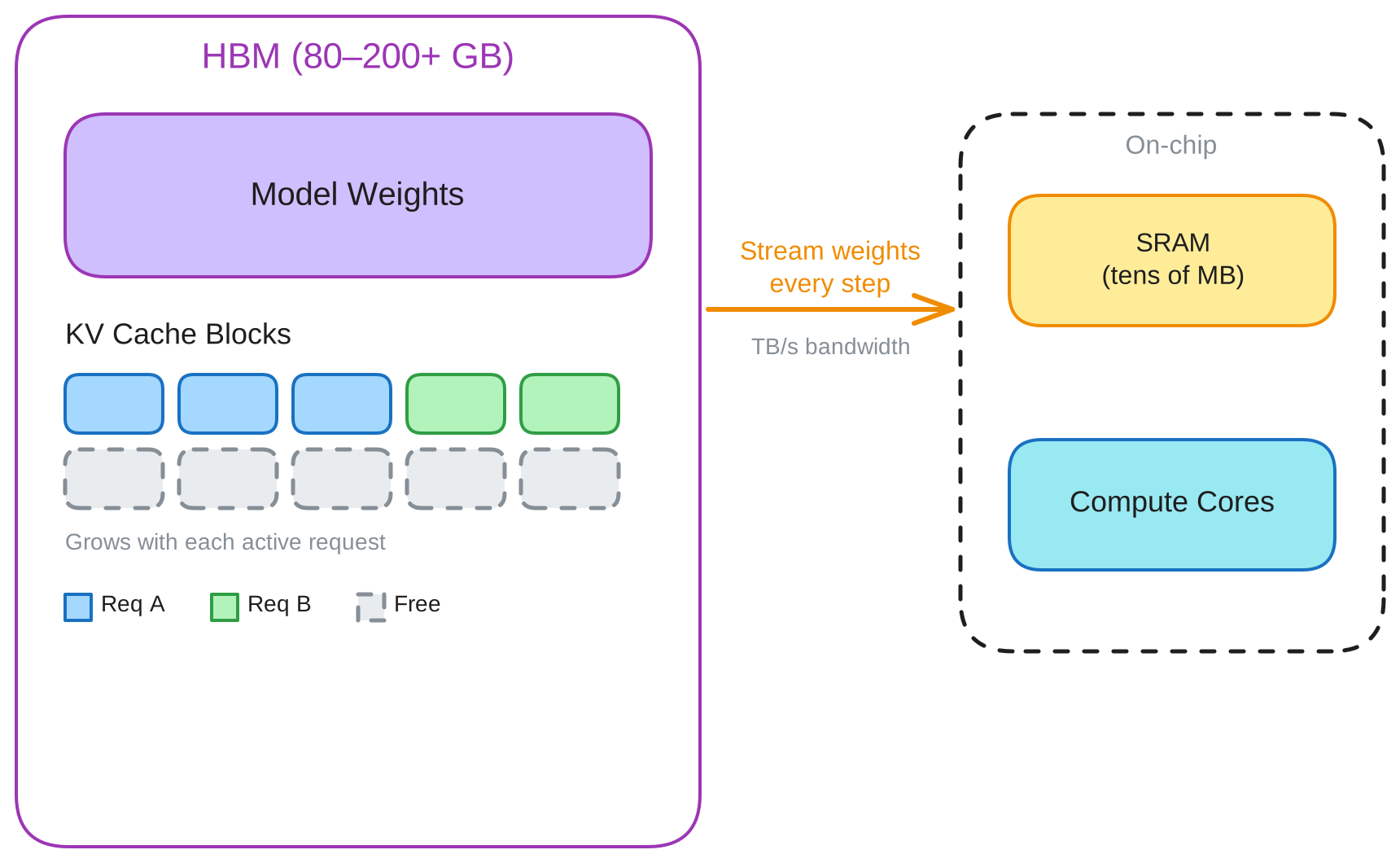
So the GPU processes the model one layer at a time. It streams Layer 1’s weights from HBM into SRAM, runs the matrix multiply, and the weights are gone, overwritten. Then it streams Layer 2’s weights, does the math, discards them. This repeats for every layer in the model.

The key thing: this happens every single step of token generation. The GPU streams the entire model through that HBM-to-SRAM pipe, produces one token per request, and then streams the entire model again for the next token. The weights pass through and get overwritten every step.

Modern inference GPUs can move data from HBM at several terabytes per second. That sounds fast, but a 13B parameter model is roughly 26 GB, and a 70B model is around 140 GB. Even at terabytes per second of bandwidth, streaming those weights takes milliseconds per step, before any KV cache reads or actual computation. That bandwidth ceiling is the thing that determines how fast decode can go.

The GPU processes the whole batch at once

Here’s the mental model shift. All requests in the current batch become rows in a matrix, and the entire GPU works on one big matrix multiply together:

Batch (4 requests in decode):        Layer weights:
[ req A token ]  ─┐
[ req B token ]   ├─── × ───── weight matrix ─────→ 4 output vectors
[ req C token ]   │
[ req D token ]  ─┘

The matrix multiply gets tiled across thousands of cores. Each core works on a piece of the overall matrix, which may span parts of multiple requests and multiple weight columns.

This has a big implication for efficiency. The GPU streams the same weights whether there’s 1 request or 32. With 1 request, you get 1 output token per weight-streaming pass. With 32 requests, you get 32 output tokens for the same pass. The weight streaming cost is fixed; only the useful work scales.

This is why batching is so effective for inference. Below a certain batch size, adding more requests is essentially free: same memory bandwidth cost, more tokens produced per step.

One step at a time

The batch is decided once at the beginning of each step. The scheduler looks at what’s waiting and what’s in progress, assigns a token count to each request, and locks in the batch. Then the GPU processes the entire batch through all layers, start to finish. Nothing changes mid-step. If a new request arrives while a step is running, it waits in a queue until the next step.

A step can mix different kinds of work. Some requests might be in their first pass (processing the full input prompt), while others are mid-generation (producing one token at a time). The scheduler handles this by giving each request the appropriate number of tokens for this step: many tokens for a new prompt, one token for an ongoing generation.

Step N:
  Scheduler: { req A: 1 token, req B: 1 token, req C: 200 tokens (new prompt) }
  → All three processed through Layer 1, Layer 2, ... Layer 24
  → A and B each get their next token, C gets its prompt processed

  (req D arrives mid-step, waits in queue)

Step N+1:
  Scheduler: { req A: 1, req B: 1, req C: 1, req D: 150 tokens (new prompt) }
  → All four processed through all layers

If a new prompt is very long, the scheduler can chunk it across multiple steps rather than processing it all at once, so that ongoing generations don’t stall waiting for a large prompt to finish.

Prefill and decode: two bottlenecks

This is where everything comes together. The same GPU hardware handles two very different operations, and the bottleneck is different for each.

Prefill is what happens when a new prompt arrives. All input tokens are known upfront, so the batch matrix has a row for every input token, hundreds or thousands of rows at once. This means matrix-matrix multiplication: lots of math per byte of weights streamed through the HBM pipe. The GPU’s compute cores are the bottleneck, not memory bandwidth. Prefill is compute-bound.

Decode is what happens during generation. Each request contributes one new token, so the batch matrix has just one row per request. This means matrix-vector multiplication: the GPU still streams all the weights and reads the full KV cache from HBM, but the actual math is a fraction of that data movement. Memory bandwidth is the bottleneck, not compute. Decode is memory-bandwidth-bound.

This split has a direct consequence for routing. TTFT (time to first token) measures prefill time. If you can skip prefill for a prompt the GPU has already seen, TTFT drops. Decode speed is determined by hardware bandwidth and is the same regardless of routing. The routing decision that matters is whether the GPU has to redo prefill work it’s already done.

Prefix caching

Prefill is where routing can make a difference: if the GPU has already processed a prompt prefix, it can skip that work entirely. The mechanism that makes this possible is prefix caching.

When a request arrives, vLLM checks whether it has already computed the KV cache for any prefix of the prompt. If the incoming prompt starts with the same system prompt as a previous request, the KV cache for that prefix is already in GPU memory. The new request reuses it and skips prefill for the shared portion entirely. The first request pays the full cost; subsequent requests with the same prefix get it for free.

This works at a prefix level, not just exact matches. A conversation at turn 5 that shares its first 200 tokens with turn 4 still benefits: the shared prefix hits cache, and only the new tokens need computation.

The prefix cache is local to each GPU server. Server A has no idea what server B has cached. If two requests with the same system prompt land on different servers, each one computes and caches the prefix independently, duplicating the work and the memory.

Cache-aware routing solves this by directing requests with the same prefix to the same server. But that creates a new problem: if all requests with a popular system prompt go to one server, that server gets overloaded while others sit idle. Cache affinity helps latency. Load concentration hurts throughput. I’ll dig into that tension in the next post.

What happens under pressure

The GPU is expensive, so you want to keep it busy. vLLM does this through continuous batching: after each decode step, the scheduler checks whether any requests have finished and removes them, then checks whether any new requests are waiting and adds them. The batch composition changes every step. Requests enter and leave the batch individually, so the GPU stays busy continuously.

This is what makes throughput scale. Below a saturation point, adding requests to the batch barely increases step time because the weight streaming cost dominates and is fixed regardless of batch size. Each additional request means more useful output per step for roughly the same cost. Above saturation, the compute starts to matter and step time grows, but the system degrades gracefully rather than hitting a wall.

The other thing to understand is preemption. Every request in the batch grows its KV cache with each token generated. Even without accepting new requests, the existing batch consumes more memory every step. If enough requests are in the decode phase generating long responses, GPU memory fills up from within the batch itself.

When that happens, vLLM has to free memory. It preempts the newest request: frees its KV cache blocks and pushes it back to the waiting queue. When that request gets rescheduled, its KV cache is gone. The GPU re-runs prefill on the full prompt plus every token it had already generated, recomputing work it already did.

This is where the router comes in. vLLM only sees its own GPU, so it accepts requests if there’s room right now, even though the existing batch might outgrow memory a few steps later. The router sees queue depth across all backends and can redirect requests to a less loaded server before any single server gets into this situation. Shedding a request at the routing layer is cheap. Letting it start, build up KV cache, and then get preempted wastes all that computation.

What’s next

This post covered the path from transformer basics to GPU execution to prefix caching: the pieces that explain why inference routing is a different problem from traditional load balancing. The GPU builds up state that can be reused. That state is local to each server. And the routing decision determines whether you get the reuse or pay the full cost again.

In the next post, I’ll build a cache-aware router, run it against real GPU backends, and measure the tradeoff directly. Prefix caching cuts time-to-first-token, but concentrating traffic on fewer servers hurts throughput. The interesting question is where the crossover happens and what controls it. The deployment manifests, benchmarking scripts, and paper breakdowns behind this post are in the companion repo.